Simple and Scalable Digital Pathology Analysis with NetApp AI


Muneer Ahmad Dedmari
 Medical imaging has undergone remarkable changes in terms of technological innovations and market expansion. It has transformed from a simple visualization apparatus to an advanced analytics tool in a state-of-the-art system for disease diagnosis. In addition to its noninvasive nature, medical imaging modalities also dramatically reduce healthcare costs and help improve patient comfort.
AI Improves Diagnosis—and Requires Massive Data
Healthcare facilities now generate and gather enormous amounts of imaging data, mostly unstructured in nature, in quantities that the industry has never seen before. It’s challenging for domain specialists to keep up with this pace, and it sometimes extends past the limit of conventional methods of analysis. Because artificial intelligence (AI), especially deep learning (DL), is good at finding patterns and identifying structures based on certain features, it meets the need to intelligently perform medical imaging analysis for diagnosis.The Siemens Healthineers AI-Rad Companion is an example in which not just one but multiple modalities are used along with AI to provide extensive diagnostics. Also, Google Health is regarded as one of the pioneers in this domain and has contributed extensively to the creation of state-of-the-art medical diagnostic solutions that are based on AI. These diagnostic solutions include lung cancer prediction and recognition of eye disease in its early stages (diabetic retinopathy).
Data is a huge part of the diagnostic AI process. The healthcare industry is dealing with heterogenous data, and in large volumes. As Eurostat reports, each year in Europe, 1 person in 13 undergoes magnetic resonance imaging (MRI), 1 person in 10 undergoes computed tomography (CT), and 1 person in 200 undergoes positron emission tomography (PET).1
Recent widespread adoption of digital pathology, such as whole slide imaging, has made it possible to digitize pathology slides into high-resolution images for better analysis. DL and machine learning (ML) are employed to automate recognition of morphological patterns and to interpret the results within minutes, ultimately decreasing the workload of pathologists.
However, whole slide images (WSIs) are very large (around 0.5GB to 2GB per slide), with a typical image resolution of 100,000x100,000 pixels. These characteristics prevent the direct application of DL approaches, mainly because of the hardware resources that are needed to facilitate learning from such high-resolution images. Intense preprocessing and planning are required before these slides can be used for training models.
In this blog post, I explore the challenges and discuss the workflow management for WSI data processing at scale and the use of DL for training models for tumor classification.
WSI Processing and DL Model Training
The adoption of AI is increasing in healthcare and life-science organizations, but its efficient implementation to harness the potential of WSI remains complex. Because of the large size and high resolution of WSIs, most DL methods don’t use the whole image as input. Instead, they generate equal-sized patches from it in a preprocessing step and later feed these patches for training. Each high-resolution image can generate hundreds to thousands of patches, depending on the patch extraction approach.
Patch generation can be a bottleneck and can slow down the whole process, however. To mitigate this slowdown, you could process each image in parallel and accelerate this step of the WSI analysis pipeline. On a single server, you could use multiple cores (multiprocessing) and further speed up the process, but you’re likely to reach the limits of the resources end, such as compute and storage. To get the most out of existing and new data that’s flowing in, you need to process data as fast and as efficiently as possible.
 You can use distributed high-performance computing (HPC) frameworks, such as Apache Spark, to accelerate the WSI preprocessing and to generate patches at scale by using multiple compute nodes. Multiple servers are processing data, so the question becomes: “What is the role of storage in such a high-data-demand case?” If data access needs are not met properly, it can easily become a bottleneck and compute nodes might starve for input data without being able to use resources to their maximum potential.
Also, for training models later, the file system should be easily accessible within the existing ML and DL frameworks and the underlying architecture (GPUs, and so on). This easy access is necessary to avoid the complexity of integrating these frameworks with the Spark environment. This approach could help separate data processing and preparation (Spark based) from the training phase (GPU based). Data scientists could then perform distributed training by using native tools without having to adapt code to work on the Spark cluster.
One simple reason to take this approach is that parallelization is occurring anyway within GPU cores (for example, CUDA) and between multiple GPUs (for example, Horovod). It also helps to separate the data engineering piece from data science, so that teams can be more focused and efficient and can work independently yet logically in sync. One way to achieve this efficiency is to have a parallel file system that provides flexibility and enables distributed workloads for preprocessing, as well as direct data access within the ML and DL frameworks.
Why the right file system and optimal storage are crucial
To support such high-performance I/O requirements, one option that comes to mind is the Hadoop Distributed File System (HDFS). However, the problem with HDFS is its complexity in creating a uniform platform to access data within a distributed computing platform and ML and DL clusters. Also, HDFS can’t be mounted directly as a local file system (virtually) and can’t be accessed within a GPU cluster as NFS.A better alternative to HDFS is BeeGFS, a parallel HPC file system. NetApp® E-Series storage with BeeGFS gives you consistent, near-real-time access to your data. To prevent bottlenecks and to support continuous high-performance workloads like AI, BeeGFS transparently spreads data across multiple servers and their back-end storage. And in addition to being open source (the basic features), BeeGFS comes with graphical administration and monitoring, unlike complex legacy open source parallel file systems.
The fact that BeeGFS is clustered indicates that the server nodes work together to deliver a single file system that can be simultaneously mounted and accessed by other server nodes, commonly known as clients. The main takeaway is that clients can see and consume this distributed file system similarly to a local file system such as NFS, XFS, or ext4. Therefore, data can be accessed as is by native ML and DL frameworks, without the need for any additional tools like data movers and without having to write manual scripts.
Workflow for Patch Generation, Training, and Inference on WSI
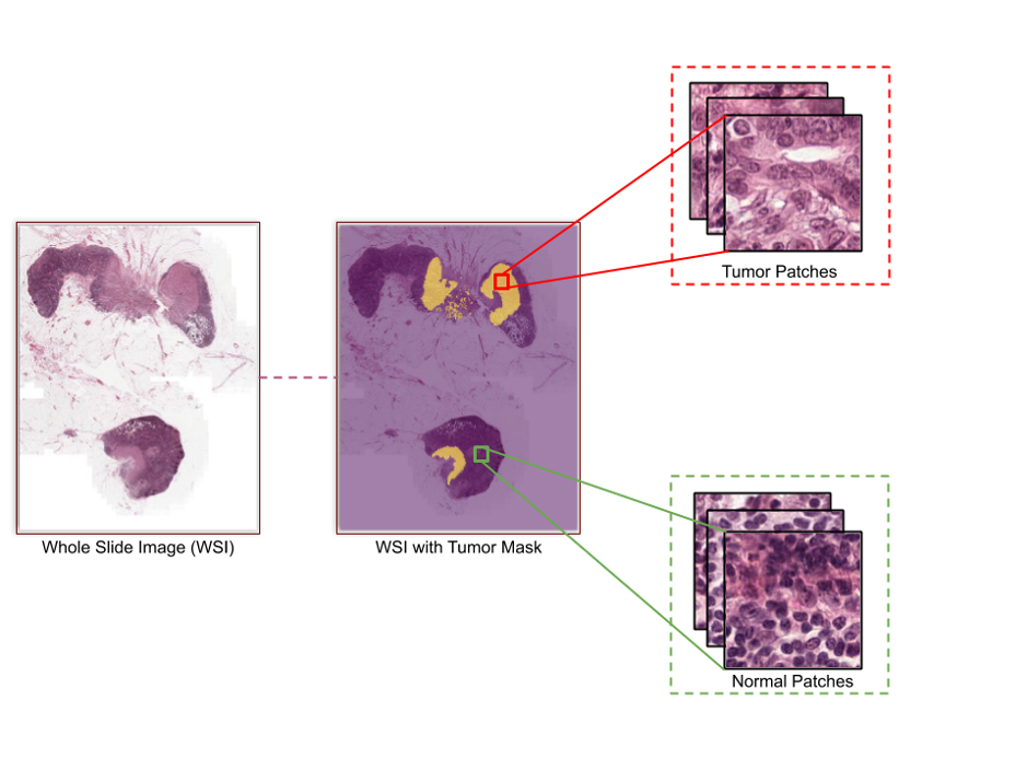
Next I will demonstrate a workflow that trains an image classification model, using native TensorFlow, to identify normal and tumor WSIs based on patches that were generated on Apache Spark. In this demonstration, we use a publicly available dataset, CAMELYON16. This dataset consists of 400 WSIs of breast cancer in TIFF format, in which 270 WSIs (160 normal and 110 with cancer metastases) are for training and 130 are for testing. The ground truth (270) is provided in XML format and consists of annotations (tumor or normal) for each training slide.
Patch generation by using Apache Spark
The ground-truth annotations consist of polygons that are stored as pixel coordinates that represent tumor regions. To extract the patches by using annotations on training slides, we need to load annotated regions per image. For simplicity and easy mapping, we use the Automated Slide Analysis Platform (ASAP) tool to create a matrix of binary masks (“0” for normal and “1” for tumor) as TIFF files from ground-truth annotations (XML). ASAP is an open source tool to visualize, to annotate, and to automatically analyze whole-slide histopathology images.We use the Apache Spark platform to generate patches in a distributed fashion on multiple compute nodes. Slides and their respective mask files are parallel-processed on different nodes, and generated patches (224x224x3) are written back as JPEG files in two different directories. One directory is for patches that consist of a tumor, and the other is for patches that do not. All data, the original WSIs and their patches, is stored in a NetApp E-Series system. E-Series provides superior performance, with low latency and high bandwidth, backed by a stable, consistent, and dynamically distributed file system (BeeGFS in this demonstration).
Training and inference for classification of “tumor” and “normal” tisues based on DL
To avoid the complexity of performing training within a Spark cluster, we perform training for classification by using native TensorFlow. It allows integration of the DL algorithms with distributed computing frameworks and makes it possible to use serverless architectures later to efficiently deploy trained models in the production environment.
Generated patches are stored as individual image files (JPEG), and loading one image at a time can create a bottleneck while training the model. We therefore create TFRecords, which make it easy to combine multiple patches in binary storage format. TFRecords are optimized for use with TensorFlow. The advantages are being able to load datasets that are too large to be stored in memory and efficient retrieval of only the data that’s required at a particular time in batches.
To train the binary classifier to predict whether the patch of a slide contains a tumor, we use an Inception-v3 architecture and load batches from TFRecords, which we created earlier. In practice, we could have a large number of WSIs and we could perform training at scale by using distributed training techniques like Horovod, where training takes place in a distributed fashion on GPU clusters.
After the training is complete, the same processing pipeline is used to create patches during inference, and the trained model is used to classify each patch as normal or as containing a tumor. We could also easily deploy models on production servers or integrate with solutions that facilitate inferencing at scale, such as NVIDIA TensorRT. We could use that approach without modifying anything in the code or the model definition, because it’s exposed as a normal model file by BeeGFS.
See It in Action Firsthand
To see how high-performance and low-latency E-Series storage facilitates WSI analysis with Apache Spark and BeeGFS, feel free to try this demonstration for yourself. You can find the setup instructions and code that we used for this demonstration on GitHub.Click to learn more about our full range of NetApp AI solutions.
Check out these additional resources:
- AI in Healthcare: Smart Infrastructure Choices Increase Success (white paper)
- Accelerate Genome Sequencing with ONTAP AI and Parabricks (solution brief)
- Three Ways AI Is Transforming the Future of Healthcare (infographic)
Muneer Ahmad Dedmari
Working as an AI Solutions Architect – Data Scientist at NetApp, Muneer Ahmad Dedmari specialized in the development of Machine Learning and Deep learning solutions and AI pipeline optimization. After working on various ML/DL projects industry-wide, he decided to dedicate himself to solutions in different hybrid multi-cloud scenarios, in order to simplify the life of Data Scientists. He holds a Master’s Degree in Computer Science with specialization in AI and Computer Vision from Technical University of Munich, Germany.